The 'Epidemiological Report' Package

Description

The EpiReport package allows the user to draft an epidemiological report similar to the ECDC Annual Epidemiological Report (AER) (see https://www.ecdc.europa.eu/en/publications-data/monitoring/all-annual-epidemiological-reports) in Microsoft Word format for a given disease.

Through standalone functions, the package is specifically designed to generate each disease-specific output presented in these reports, using ECDC Atlas export data.

Package details below:

Package	Description
Version	1.0.4
Published	2025-04-18
Authors	Lore Merdrignac l.merdrignac@epiconcept.fr, Author of the package and original code Tommi Karki tommi.karki@ecdc.europa.eu, Esther Kissling e.kissling@epiconcept.fr, Joana Gomes Dias joana.gomes.dias@ecdc.europa.eu, Project manager
Maintainer	Lore Merdrignac l.merdrignac@epiconcept.fr
License	EUPL
Link to the ECDC AER reports	https://www.ecdc.europa.eu/en/publications-data/monitoring/all-annual-epidemiological-reports

https://epiconcept-paris.github.io/EpiReport/

Background

ECDC’s annual epidemiological report is available as a series of individual epidemiological disease reports. Reports are published on the ECDC website https://www.ecdc.europa.eu/en/publications-data/monitoring/all-annual-epidemiological-reports as they become available.

The year given in the title of the report (i.e. ‘Annual epidemiological report for 2016’) refers to the year the data were collected. Reports are usually available for publication one year after data collection is complete.

All reports are based on data collected through The European Surveillance System (TESSy)¹ and exported from the ECDC Atlas. Countries participating in disease surveillance submit their data electronically.

The communicable diseases and related health issues covered by the reports are under European Union and European Economic Area disease surveillance² ³ ⁴ ⁵.

ECDC’s annual surveillance reports provide a wealth of epidemiological data to support decision-making at the national level. They are mainly intended for public health professionals and policymakers involved in disease prevention and control programmes.

1. Datasets to be used in the Epidemiological Report package

1.1. Disease dataset specification

Two types of datasets can be used:

The default dataset included in the EpiReport package which includes Salmonellosis data for 2012-2016: EpiReport::SALM2016;
Any dataset specified as described below.

Description of each variable required in the disease dataset (naming and format):

HealthTopicCode: Character string, disease code (see also the reports parameter table Tab.3);
MeasurePopulation: Character string, population characteristics (e.g. All cases, Confirmed cases, Serotype AGONA, Serotype BAREILLY etc.).
MeasureCode: Character string, code of the indicators available (e.g. ALL.COUNT, ALL.RATE, CONFIRMED.AGESTANDARDISED.RATE etc.);
TimeUnit: Character string, unit of the time variable TimeCode (e.g. M for monthly data, Y for yearly data).
TimeCode: Character string, time variable including dates in any formats available i.e. yearly data (e.g. 2001) or monthly data (e.g. 2001-01);
GeoCode: Character string, geographical level in coded format (e.g. AT for Austria, BE for Belgium, BG for Bulgaria, see also the EpiReport::MSCode table, correspondence table for Member State labels and codes);
XLabel: The label associated with the x-axis in the epidemiological report (see getAgeGender() and plotAgeGender() bar graph for the age variable);
YLabel: The label associated with the y-axis in the epidemiological report (see getAgeGender() and plotAgeGender() bar graph for the grouping variable gender);
ZValue: The value associated with the stratification of XLabel and YLabel in the age and gender bar graph (see getAgeGender() and plotAgeGender());
YValue: The value associated with the y-axis in the epidemiological report (see plotAge bar graph for the variable age, or getTableByMS() for the number of cases, rate or age-standardised rate in the table by Member States by year);
N: Integer, number of cases (see getTrend() and getSeason() line graph).

**Tab.1 Example of Salmonellosis data 2012-2016**
HealthTopicCode	MeasurePopulation	MeasureCode	TimeUnit	TimeCode	GeoCode	XLabel	YLabel	ZValue	YValue	N
SALM	Confirmed cases	CONFIRMED.GENDER.PROPORTION	M	2015-04	MT	Female	NA	NA	16.6666667	6
SALM	Confirmed cases	CONFIRMED.AGE.RATE	M	2013-06	EE	15-24	NA	NA	10.8818107	44
SALM	Confirmed cases	CONFIRMED.AGE.COUNT	M	2016-08	HU	65+	NA	NA	105.0000000	705
SALM	Confirmed cases	CONFIRMED.AGE.PROPORTION	M	2014-12	FR	0-4	NA	NA	28.9879931	585
SALM	Confirmed cases	CONFIRMED.GENDER.COUNT	Y	2015	IT	Male	NA	NA	2070.0000000	3825
SALM	Confirmed cases	CONFIRMED.AGE.RATE	M	2013-04	CZ	65+	NA	NA	2.7720922	405
SALM	Confirmed cases	CONFIRMED.AGE.PROPORTION	M	2013-10	EE	65+	NA	NA	22.2222222	18
SALM	Confirmed cases	CONFIRMED.AGE.RATE	M	2015-12	BE	15-24	NA	NA	1.0574370	191
SALM	Confirmed cases	CONFIRMED.AGE.RATE	M	2014-07	NL	5-14	NA	NA	0.5602065	69
SALM	Confirmed cases	CONFIRMED.AGE_GENDER.RATE	Y	2014	EE	45-64	Female	4.29461	2.0000000	92

1.2. Report parameters dataset specification

The internal dataset EpiReport::AERparams describes the parameters to be used for each output of each disease report.

If the user wishes to set different parameters for one of the 53 covered health topics, or if the user wishes to analyse an additional disease not covered by the default parameter table, it is possible to use an external dataset as long as it is specified as described below and in the help page ?EpiReport::AERparams. All functions of the EpiReport package can then be fed with this specific parameter table.

List of the main parameters included:

HealthTopic: Character string, disease code that should match with the health topic code from the disease-specific dataset (see Tab.1)
MeasurePopulation: Character string, population to present in the report: either ALL cases or CONFIRMED cases only.
TableUse: Character string, specifying whether to include the table in the epidemiological report and which table to include:
- NO: No table included
- COUNT: Table presenting the number of cases by Member State by year
- RATE: Table presenting the rates of cases by Member State by year
- ASR: Table presenting the age-standardised rates of cases by Member State by year
AgeGenderUse: Character string, specifying whether to include the age and gender bar graph in the epidemiological report and which type of graph to include:
- NO: No graph included
- AG-COUNT: Bar graph presenting the number of cases by age and gender
- AG-RATE: Bar graph presenting the rates of cases by age and gender
- AG-PROP: Bar graph presenting the proportion of cases by age and gender
- A-RATE: Bar graph presenting the rates of cases by age
TSTrendGraphUse: Yes/No, specifying whether to include a line graph describing the trend of the disease over the time.
TSSeasonalityGraphUse: Yes/No, specifying whether to include a line graph describing the seasonality of the disease.
MapNumbersUse: Yes/No, specifying whether to include the map presenting the number of cases by Member State.
MapRatesUse: Yes/No, specifying whether to include the map presenting the rates of cases by Member State.
MapASRUse: Yes/No, specifying whether to include the map presenting the age-standardised rates of cases by Member State.

**Tab.2 Example of the main columns of the parameter dataset**
HealthTopic	MeasurePopulation	TableUse	AgeGenderUse	TSTrendGraphUse	TSSeasonalityGraphUse	MapNumbersUse	MapRatesUse	MapASRUse
ZIKV	ALL	COUNT	AG-PROP	N	N	Y	N	N
LEGI	ALL	ASR	AG-RATE	Y	Y	N	Y	N
TUBE	ALL	ASR	AG-RATE	N	N	N	Y	N
CCHF	ALL	COUNT	NO	N	N	N	N	N
SYPH	CONFIRMED	RATE	AG-RATE	N	N	N	Y	N

1.3. Member States correspondence table dataset

The internal dataset EpiReport::MSCode provides the correspondence table of the geographical code GeoCode used in the disease dataset, and the geographical label Country to use throughout the report. Additional information on the EU/EEA affiliation is also available in column EUEEA.

**Tab.3 Example of geographical codes and associated labels**
Country	GeoCode	EUEEA	TheCountry
Czechia	CZ	EU	Czechia
United Kingdom	UK	EU	the United Kingdom
Croatia	HR	EU	Croatia
Italy	IT	EU	Italy
Belgium	BE	EU	Belgium

2. How to generate the Epidemiological Report in Microsoft Word format

To generate a similar report to the Annual Epidemiological Report, we can use the default dataset included in the EpiReport package presenting Salmonellosis data 2012-2016.

Calling the function getAER(), the Salmonellosis 2016 report will be generated and stored in your working directory (see getwd()) by default.

getAER()

Please specify the full path to the output folder if necessary:

output <- "C:/EpiReport/doc/"
getAER(outputPath = output)

2.1. External disease dataset

To generate the report using an external dataset, please use the syntax below.

In the following example, Pertussis 2016 TESSy data (in csv format, in the /data folder) is used to produce the corresponding report.

Pertussis PNG maps have previously been created and stored in a specific folder /maps.

# --- Importing the dataset
PERT2016 <- read.table("data/PERT2016.csv", 
                       sep = ",", 
                       header = TRUE, 
                       stringsAsFactors = FALSE)

# --- Specifying the folder containing pertussis maps
pathMap <- paste(getwd(), "/maps", sep = "")


# --- (optional) Setting the local language in English for month label
Sys.setlocale("LC_TIME", "C")
#> [1] "C"

# --- Producing the report
EpiReport::getAER(disease = "PERT", 
       year = 2016, 
       x = PERT2016, 
       pathPNG = pathMap)

Please note that the font Tahoma is used in the plot axis and legend. It is advised to import this font using the extrafont package and the command font_import and loadfonts.

However, if the users prefer the use of the default Arial in plots, it is optional. In that case, warnings will appear in the console for each plot.

2.2. Word template

By default, an empty ECDC template (Microsoft Word) is used to produce the report. In order to modify this template, please first download the default template using the function getTemplate().

You can store this Microsoft Word template in a specific folder /template.

getTemplate(output_path = "C:/EpiReport/template")

Then, apply the modifications required, save it and use it as a new Microsoft Word template when producing the epidemiological report as described below.

getAER(template = "C:/EpiReport/template/New_AER_Template.docx",
       outputPath = "C:/EpiReport/doc/")

Please make sure that the Microsoft Word bookmarks are preserved throughout the modifications to the template. The bookmarks specify the location where to include each output.

2.3. Word bookmarks

Each epidemiological output will be included in the Word template in the corresponding report chapter. The EpiReport package relies on Microsoft Word bookmarks to specify the exact location where to include each output.

The list of bookmarks recognised by the EpiReport package are:

YEAR
DISEASE
DATEPUBLICATLAS
TABLE1_CAPTION
TABLE1
MAP_NB_CAPTION
MAP_NB
MAP_RATE_CAPTION
MAP_RATE
MAP_ASR_CAPTION
MAP_ASR
TS_TREND_CAPTION
TS_TREND
TS_TREND_COUNTRIES
TS_SEASON_CAPTION
TS_SEASON
TS_SEASON_COUNTRIES
BARGPH_AGEGENDER_CAPTION
BARGPH_AGEGENDER
BARGPH_AGE_CAPTION
BARGPH_AGE

3. How to generate each epidemiological outputs independently

The EpiReport package allows the user to generate each epidemiological output independently of the Microsoft Word report.

The ECDC annual epidemiological Report includes five types of outputs:

Table: Distribution of cases by Member State over the last five years with:
- the number of cases only;
- the number of cases and the corresponding rate per 100 000 population or
- the number of cases, the rate and the age-standardised rate per 100 000 population.
Seasonality plot: Distribution of cases at EU/EEA level, by month, over the past five years.
Trend plot: Trend and number of cases at EU/EEA level, by month, over the past five years.
Map: Distribution of cases by Member State presenting either:
- the number of cases;
- the rates per 100 000 population;
- the age-standardised rates per 100 000 population.
Age and gender bar graph: Distribution of cases at EU/EEA level:
- by age and gender and using:
  - the number of cases
  - the rate
  - the proportion of cases
- by age only and using the rate.

3.1. Table: distribution of cases by Member State

The function getTableByMS() generates a flextable object (see package flextable) presenting the number of cases by Member State over the last five years.

By default, the function will use the internal Salmonellosis 2012-2016 data and present the number of confirmed cases and the corresponding rate for each year, with a focus on 2016 and age-standardised rates.

EpiReport::getTableByMS()

Country	2015		2016		2017		2018		2019
Country	Number	Rate	Number	Rate	Number	Rate	Number	Rate	Number	Rate	ASR
Austria	103	1.2	116	1.3	85	1.0	85	1.0	142	1.6	1.7
Belgium	108	1.0	114	1.0	77	0.7	101	0.9	202	1.8	1.9
Bulgaria	.	.	.	.	.	.	.	.	.	.	.
Croatia	-	-	2	0.0	0	0.0	2	0.0	4	0.1	0.1
Cyprus	.	.	.	.	.	.	.	.	.	.	.
Czechia	0	0.0	0	0.0	0	0.0	0	0.0	0	0.0	0.0
Denmark	.	.	.	.	.	.	.	.	.	.	.
Estonia	12	0.9	9	0.7	8	0.6	6	0.5	6	0.5	0.5
Finland	54	1.0	66	1.2	25	0.5	56	1.0	81	1.5	1.6
France	285	0.4	373	0.6	266	0.4	331	0.5	904	1.3	1.4
Germany	722	0.9	958	1.2	635	0.8	614	0.7	1175	1.4	1.5
Greece	2	0.0	2	0.0	1	0.0	2	0.0	10	0.1	0.1
Hungary	12	0.1	24	0.2	17	0.2	14	0.1	44	0.5	0.5
Iceland	0	0.0	0	0.0	1	0.3	1	0.3	4	1.1	1.1
Ireland	8	0.2	18	0.4	10	0.2	17	0.4	18	0.4	0.4
Italy	103	0.2	106	0.2	95	0.2	108	0.2	231	0.4	0.4
Latvia	4	0.2	9	0.5	13	0.7	12	0.6	11	0.6	0.6
Liechtenstein	.	.	.	.	.	.	.	.	.	.	.
Lithuania	9	0.3	4	0.1	4	0.1	8	0.3	9	0.3	0.4
Luxembourg	0	0.0	1	0.2	0	0.0	1	0.2	1	0.2	0.2
Malta	1	0.2	1	0.2	3	0.7	1	0.2	2	0.4	0.4
Netherlands	18	-	6	-	0	-	0	-	0	-	-
Norway	98	1.9	64	1.2	35	0.7	49	0.9	102	1.9	2.0
Poland	12	0.0	41	0.1	29	0.1	30	0.1	55	0.1	0.1
Portugal	14	0.1	13	0.1	11	0.1	14	0.1	30	0.3	0.3
Romania	7	0.0	8	0.0	7	0.0	4	0.0	15	0.1	0.1
Slovakia	2	0.0	4	0.1	2	0.0	7	0.1	6	0.1	0.1
Slovenia	3	0.1	6	0.3	5	0.2	8	0.4	21	1.0	1.1
Spain	168	0.4	261	0.6	128	0.3	205	0.4	228	0.5	0.5
Sweden	159	1.6	225	2.3	106	1.1	106	1.0	235	2.3	2.4
United Kingdom	423	0.7	468	0.7	465	0.7	432	0.7	827	1.2	1.3
EU-EEA	2327	0.5	2899	0.6	2028	0.4	2214	0.5	4363	0.9	0.9

Table. Distribution of confirmed salmonellosis cases, EU/EEA, 2012-2016

This table can be drafted using external data, and specifying the disease code and the year to use as reference in the report.

In the example below, we use Zika virus data. According to the report parameters, the table for this disease should present the number of reported cases over the last five years and by Member State.

ZIKV2016 <- read.table("data/ZIKV2016.csv", 
                       sep = ",", 
                       header = TRUE, 
                       stringsAsFactors = FALSE)
EpiReport::getTableByMS(x = ZIKV2016, 
             disease = "ZIKV", 
             year = 2016)

Country	2012	2013	2014	2015	2016
Country	Number		Number		Number
Austria	-	-	-	1	41
Belgium	-	-	-	1	120
Bulgaria	.	.	.	.	.
Croatia	.	.	.	.	.
Cyprus	.	.	.	.	.
Czechia	-	-	-	-	13
Denmark	-	-	-	-	8
Estonia	-	-	-	-	0
Finland	-	-	-	1	6
France	-	-	-	-	1141
Germany	.	.	.	.	.
Greece	-	-	-	-	4
Hungary	-	-	-	-	2
Iceland	.	.	.	.	.
Ireland	-	-	-	1	15
Italy	-	-	-	-	101
Latvia	0	0	0	0	0
Liechtenstein	.	.	.	.	.
Lithuania	.	.	.	.	.
Luxembourg	-	-	-	-	2
Malta	-	-	-	-	2
Netherlands	-	-	-	11	98
Norway	-	-	-	-	8
Poland	.	.	.	.	.
Portugal	-	-	-	-	18
Romania	-	-	-	-	3
Slovakia	-	-	-	-	3
Slovenia	-	-	-	-	7
Spain	-	-	-	10	301
Sweden	-	-	-	1	34
United Kingdom	-	-	-	3	194
EU-EEA	0	0	0	29	2121

Table. Distribution of Zika virus infection cases, EU/EEA, 2012-2016

3.2. Seasonality plot: distribution of cases by month

The function getSeason() generates a ggplot (see package ggplot2) presenting the distribution of cases at EU/EEA level, by month, over the past five years.

The plot includes:

The number of cases by month in the reference year (green solid line)
The mean number of cases by month in the four previous years (grey dashed line)
The minimum number of cases by month in the four previous years (grey area)
The maximum number of cases by month in the four previous years (grey area)

By default, the function will use the internal Salmonellosis 2012-2016 data.

# --- Salmonellosis 2016 plot
EpiReport::getSeason()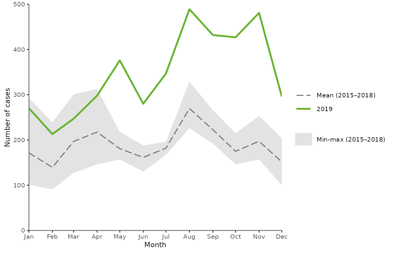

Figure. Distribution of confirmed salmonellosis cases by month, EU/EEA, 2016 and 2012-2015

The plot can also be drafted using external data, and specifying the disease dataset, the disease code and the year to use as reference in the report.

In the example below, we use Pertussis 2012-2016 data.

# --- Pertussis 2016 plot
EpiReport::getSeason(x = PERT2016,
                     disease = "PERT",
                     year = 2016)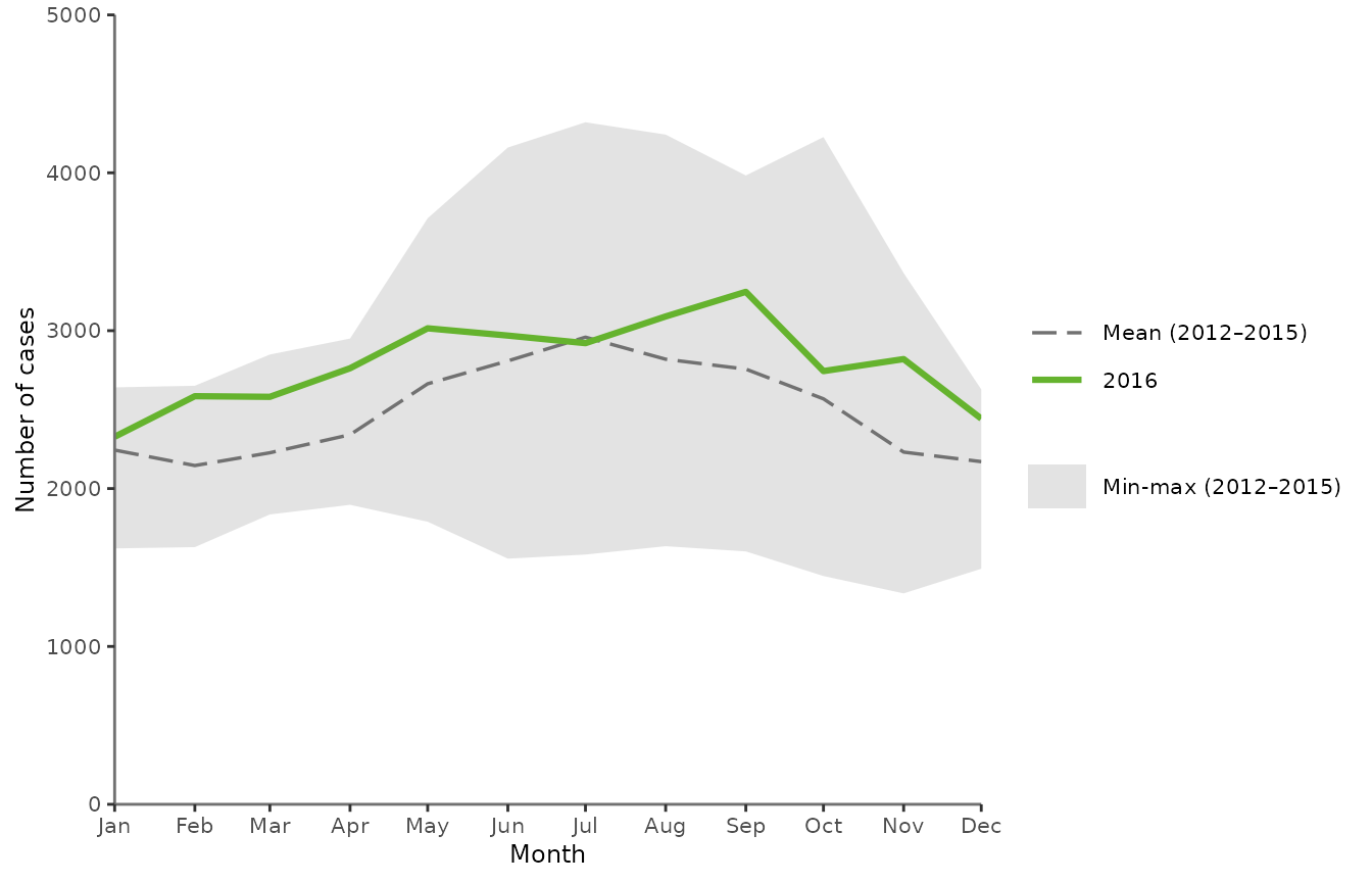

Figure. Distribution of pertussis cases by month, EU/EEA, 2016 and 2012-2015

3.3. Trend plot: trend and number of cases by month

The function getTrend() generates a ggplot (see package ggplot2) presenting the trend and the number of cases at EU/EEA level, by month, over the past five years.

The plot includes:

The number of cases by month over the 5-year period (grey solid line)
The 12-month moving average of the number of cases by month (green solid line)

By default, the function will use the internal Salmonellosis 2012-2016 data.

# --- Salmonellosis 2016 plot
EpiReport::getTrend()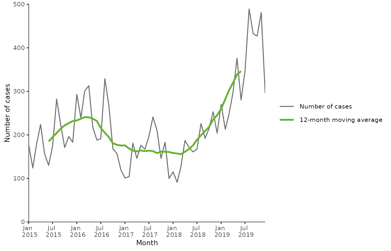

Figure. Trend and number of confirmed salmonellosis cases, EU/EEA by month, 2012-2016

The plot can also be drafted using external data, and specifying the disease dataset, the disease code and the year to use as reference in the report.

In the example below, we use again Pertussis 2012-2016 data.

# --- Pertussis 2016 plot
EpiReport::getTrend(x = PERT2016,
                    disease = "PERT",
                    year = 2016)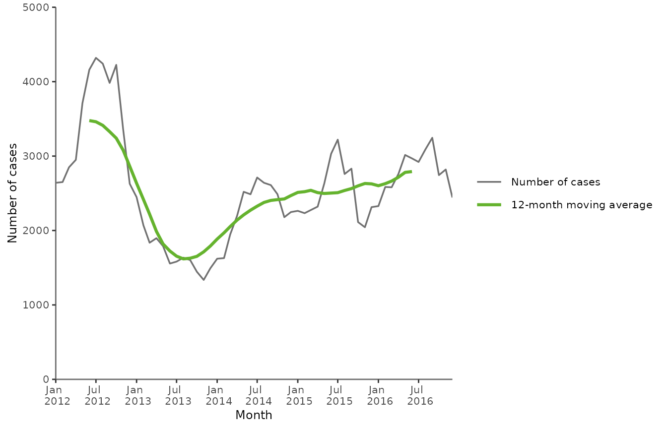

Figure. Trend and number of pertussis cases, EU/EEA by month, 2012-2016

3.4. Maps: distribution of cases by Member State

The function getMap() provides with a preview of the PNG map associated with the disease.

By default, the function will use the internal Salmonellosis 2016 PNG maps. According to the report parameters, the corresponding map should present the notification rate of confirmed salmonellosis cases.

# --- Salmonellosis 2016 map
EpiReport::getMap()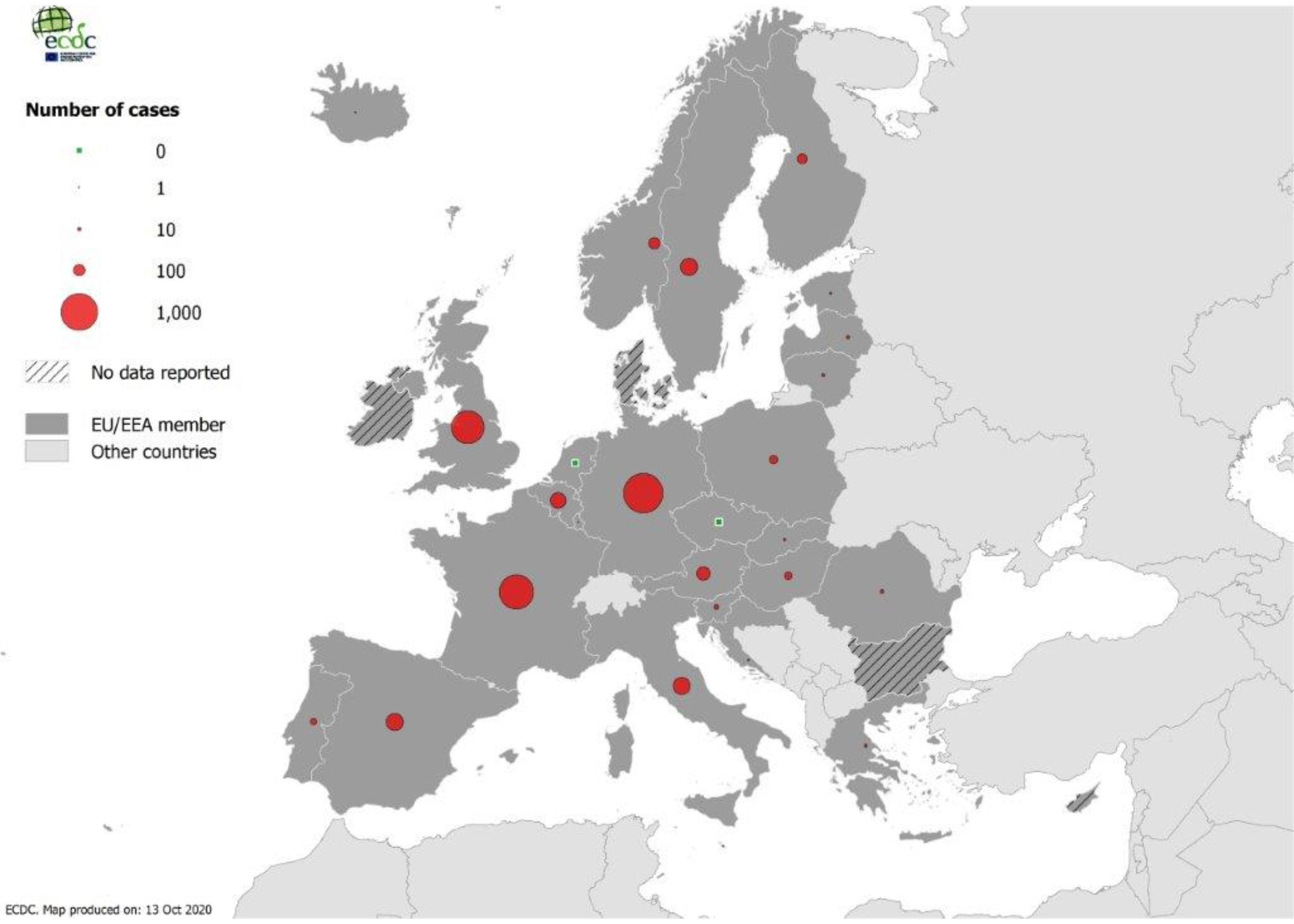

Figure. Distribution of confirmed salmonellosis cases per 100 000 population by country, EU/EEA, 2016

The map can also be included using external PNG files, and specifying the disease code and the year to use as reference in the report. The corresponding syntax is described below (pertussis map not available).

# --- Pertussis 2016 map
EpiReport::getMap(disease = "PERT", 
                  year = 2016, 
                  pathPNG = "C:/EpiReport/maps/")

3.5. Age and gender bar graph

The function getAgeGender() generates a ggplot (see package ggplot2) presenting in a bar graph the distribution of cases at EU/EEA level by age and gender.

The bar graph uses either:

The number of cases,
The rate per 100 000 cases,
The proportion of cases.

By default, the function will use the internal Salmonellosis 2012-2016 data with the rate of confirmed cases per 100 000 population.

# --- Salmonellosis 2016 bar graph
EpiReport::getAgeGender()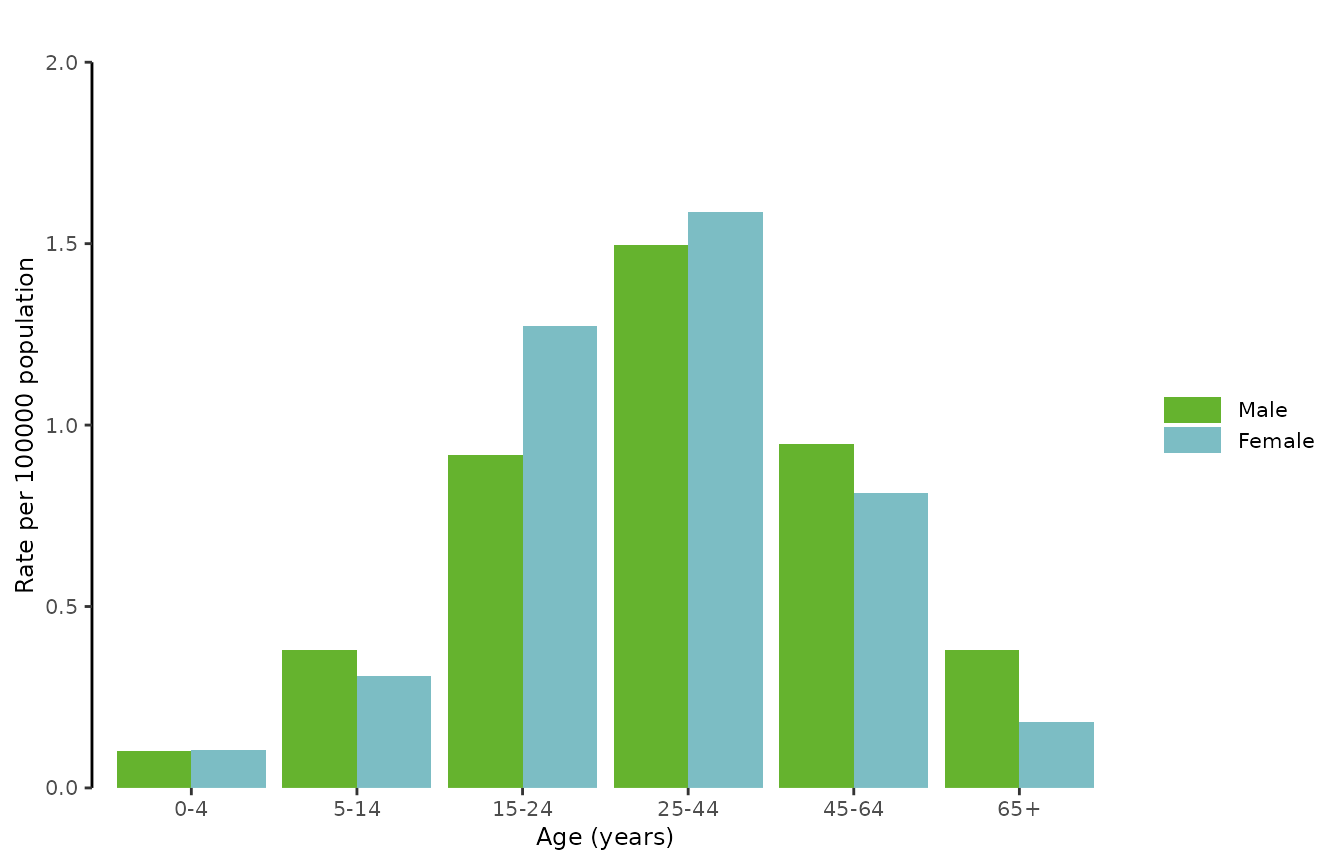

Figure. Distribution of confirmed salmonellosis cases per 100 000 population, by age and gender, EU/EEA, 2016

The bar graph can also be drafted using external data, and specifying the disease dataset, the disease code and the year to use as reference in the report.

In the example below, we use Zika 2012-2016 data.

# --- Zika 2016 bar graph
EpiReport::getAgeGender(x = ZIKV2016, 
                        disease = "ZIKV", 
                        year = 2016)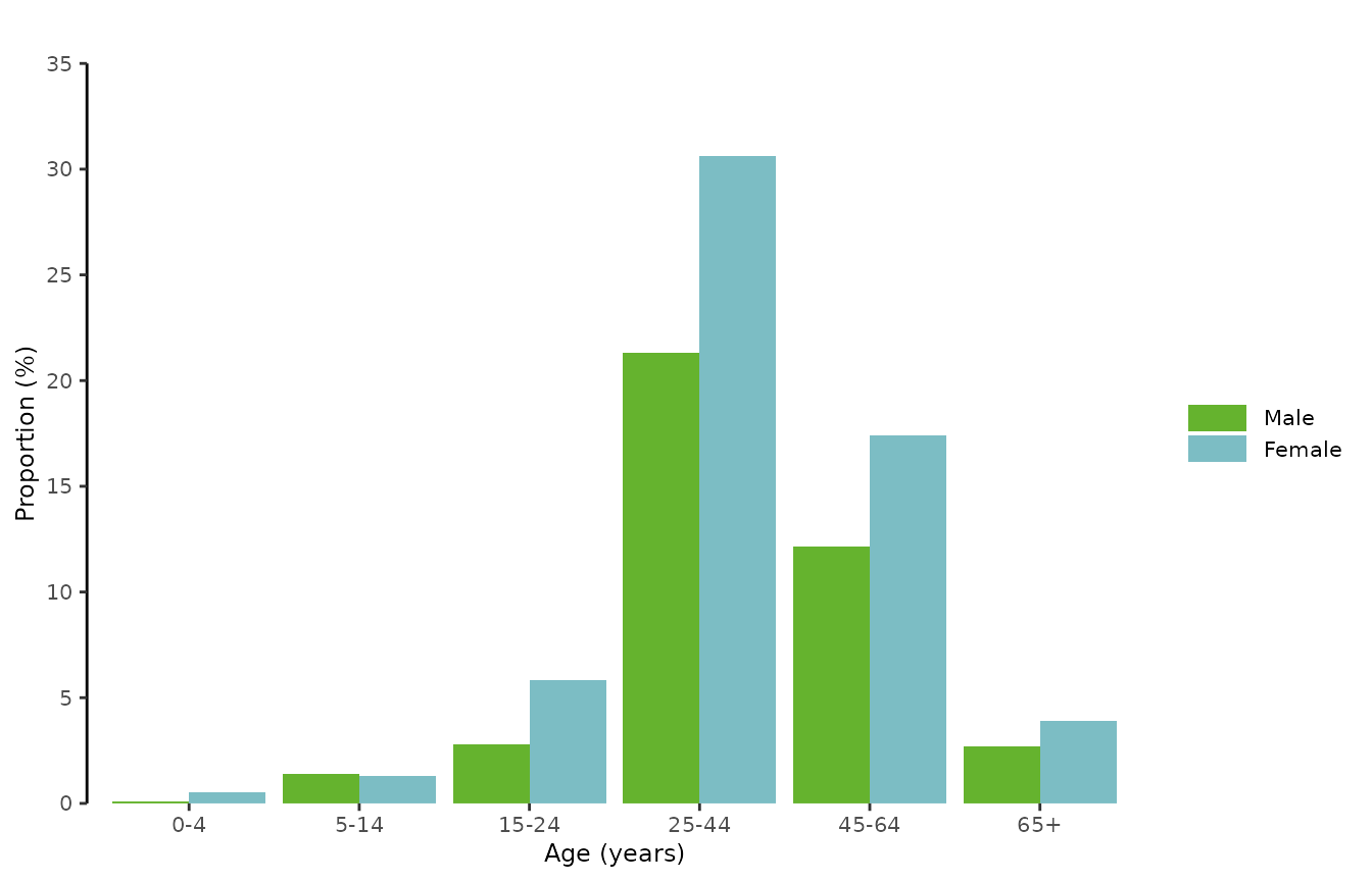

Figure. Distribution of Zika virus infection proportion (%), by age and gender, EU/EEA, 2016

European Centre for Disease Prevention and Control (ECDC)